TRIC-seq explorer guide

Overview: What is TRIC-seq?

TRIC-seq (Total RNA Interactome Capture) is an in situ, genetics‑free proximity‑ligation method that maps native RNA–RNA contacts across bacterial transcriptomes. It preserves cellular context and resolves both intramolecular (structure) and intermolecular (regulatory/proximity) contacts at high resolution and specificity.

Each chimeric read corresponds to one ligation event between two RNA fragments that were nearby in the cell. Aggregating millions of such events resolves:

RNA structures (Hi‑C–like self‑contact maps, identifying functional domains, insulators, and structural hot-spots).
Regulatory networks (identifying highly connected sRNA–mRNA pairs, regulatory sponges, and trans-acting hubs).
System‑level patterns (uncovering modular interactomes, extensive mRNA-mRNA contacts, and condensate‑like organization, driven largely by non-ribosomal transcripts).

Biological Insights

By circumventing biases associated with probe-based or UV-crosslinking strategies, TRIC-seq provides an unbiased look into the spatial orchestration of the transcriptome. Key findings unlocked by TRIC-seq include:

Pervasive mRNA-mRNA architecture: Transcripts don't act alone; they frequently overlap geographically, participating in interconnected communities and operon-spanning regulatory cross-talk.
Target discovery: Novel trans-acting RNA-RNA interactions can be discovered systematically by mapping robustly enriched intermolecular loops (significant Odd Ratios).
Tertiary folds in vivo: Long-range intramolecular contacts pinpoint 5′UTR/3′UTR interactions that gate functional expression.

Reference: Comprehensive architecture of the bacterial RNA interactome (preprint).

Using this dataset

The Explorer ships with pre‑loaded TRIC‑seq datasets for multiple bacteria — Escherichia coli (K‑12 MG1655, the reference interactome), Staphylococcus aureus, Stutzerimonas stutzeri and Myxococcus xanthus — plus a self‑consistent simulated demo you can click through instantly. Pick any of them from the dataset menu (top‑right).

Key fields

Interaction count (i_o): unique chimeric reads supporting a pair.
Odds ratio (O^f): enrichment relative to a null; higher means more specific pairing.
Adjusted P/FDR: multiple‑testing–corrected significance (especially for long‑range contacts).
Feature types: 5′UTR, CDS, 3′UTR, sRNA, tRNA, housekeeping RNA (hkRNA), sponge.

Quick start

Open the Explorer and choose a species (or the demo) from the dataset menu.
Search any RNA in the top bar (⌘K), e.g. sRNA RyhB or CDS uvrA. It becomes the focal RNA.
Read its partners in the right‑hand panel; tune filters (min i_o and O^f).
Click any partner to refocus on it; double‑click to open its Pair contact map.

Recommended starting thresholds (E. coli, trans): O^f ≥ 10 and i_o ≥ 5. Loosen to explore; tighten for high‑confidence sets. For highly connected RNAs (e.g., rRNAs), prioritize O^f/FDR over raw counts.

From the preprint—practical reading tips:

TRIC‑seq simultaneously captures intramolecular structure signals and intermolecular regulatory contacts; interpret diagonal‑proximal self‑contacts as structure and distal cross‑locus contacts as pairing/regulatory proximity.
Contact specificity is better reflected by O^f (and FDR) than by counts alone—use both when ranking candidates.
Use long‑range (kb‑scale) enrichment to flag distal regulation, then validate in the Pair lens.

Cite this resource: please cite the TRIC‑seq preprint doi:10.1101/2025.09.11.675593 and GEO accession GSE305265 when using this explorer.

Recommended

The Explorer — one RNA, every lens

The Explorer unifies all four legacy tools into a single workspace. You pick one focal RNA and view it through four lenses that all read from the same dataset and the same filters. Change the focal RNA and every lens updates at once — so you can move from a genome‑wide overview to a base‑pair‑level interface without losing your place.

Interactome≈ globalMAP

Every partner of the focal RNA, on a circular genome or a linear scatter.

Pair≈ pairMAP

A base‑pairing contact map between the focal RNA and one chosen partner, with built‑in duplex prediction.

Structure≈ foldMAP

The focal RNA's intramolecular self‑contact map and its long‑range contact profile.

Compare≈ csMAP

The focal RNA's target spectrum lined up against pinned RNAs.

Anatomy of the workspace

Five regions you'll use constantly. Numbers below match the figure.

Annotated map of the Explorer workspace — The Explorer workspace: ① focal‑RNA search, ② shared filters & dataset menu, ③ lens tabs, ④ the active lens, ⑤ the partners panel.

Focal‑RNA search — type any gene/RNA name (or press ⌘K / Ctrl K), arrow‑keys to choose, Enter to set the focal RNA.
Filters & dataset — the sliders icon opens shared filters (below); the dataset button switches species, loads the demo, or uploads your own data.
Lens tabs — switch between Interactome / Pair / Structure / Compare. The Compare tab shows a badge with the number of RNAs you've pinned.
Active lens — the main canvas. Every plot has an Export PNG button.
Partners panel — a live, sortable list of the focal RNA's partners with pin / pair / database‑link actions, CSV export and an AI‑hypothesis helper.

Shared filters

One set of filters applies to every lens, so a threshold you set in the Interactome also shapes the partner list and the Compare spectra.

Control	Default	What it does
Min reads (i_o)	5	Hide partners supported by fewer unique chimeric reads.
Odds‑ratio cap (O^f)	5000	Clamp the plotted odds ratio so a few huge values don't flatten the scale (data is not removed).
Label threshold	50	Only partners with O^f above this get a text label in the maps.
Circle size	×1	Scale every dot up or down for crowded or sparse RNAs.
Exclude feature types	tRNA off	Toggle whole classes (5′UTR, CDS, 3′UTR, sRNA/ncRNA, rRNA/hkRNA, sponge, tRNA) in or out.
Highlight genes	—	Type names (comma/space‑separated) to make those partners glow yellow across the maps.

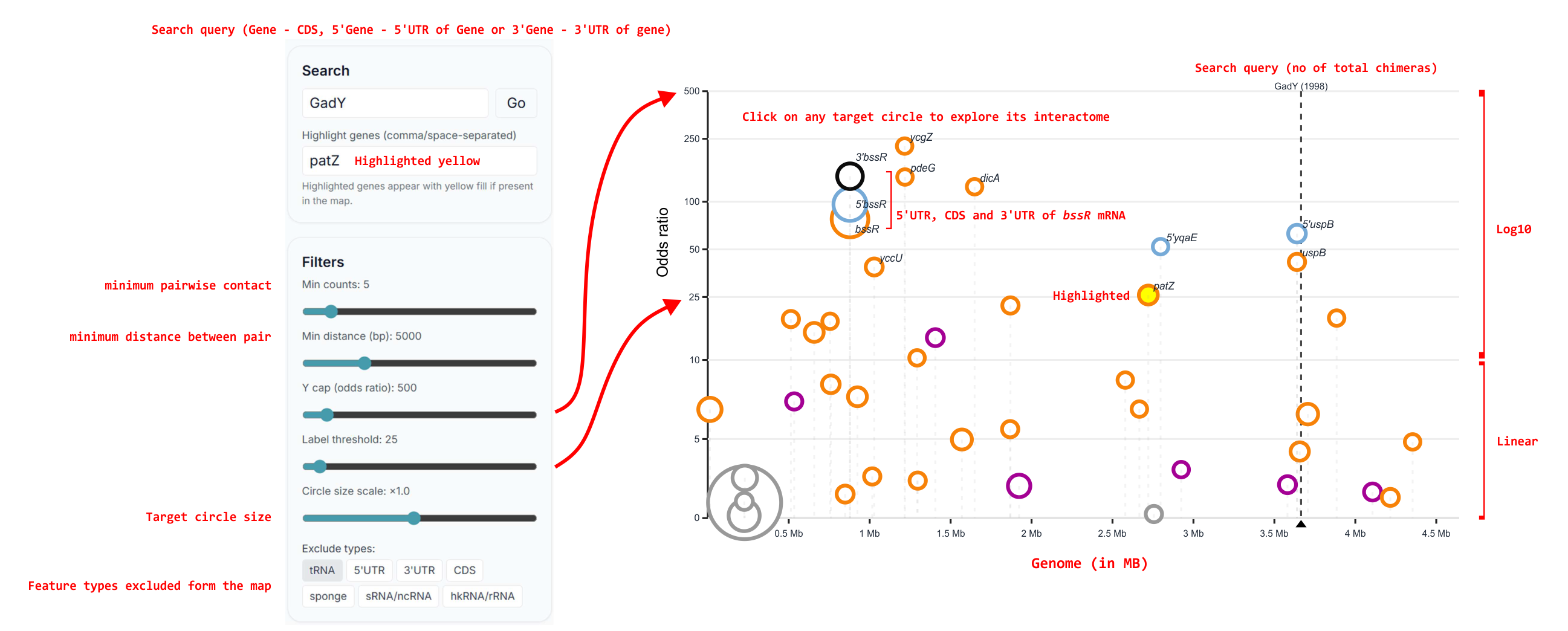
The golden rule: click a partner to refocus the whole Explorer on it; double‑click to open its Pair map. This works in the Interactome map and in the partners list, and is the fastest way to walk an interaction network hop by hop.

Interactome lens ≈ globalMAP

What it shows: a genome‑aware, RNA‑centric map of all partners of the focal RNA. The focal RNA sits at the centre; each partner is drawn at its real genomic position. Dot area ∝ reads (i_o), dot outline = feature type, and the connecting arc's colour encodes the odds ratio (O^f).

Interactome lens — circular genome view of the sRNA GcvB and its partners in E. coli — Interactome (Genome view) of the sRNA *GcvB* in *E. coli*. Chords fan out from the focal RNA to each partner; arc colour = odds ratio, arc width = read depth, dot area = reads, dot outline = feature class. GcvB's top partners are the 5′UTRs of its amino‑acid–transport regulon (*oppA*, *dppA*, *argT*, *sstT*…).

Interactome with the RIL-seq overlay — GcvB partners that are known RIL-seq targets shown in teal — The same view with the **RIL‑seq overlay** on. Teal chords/dots mark partners that are independently known RIL‑seq targets (Melamed et al. 2016); the button reads **RIL‑seq (19)** — here every one of GcvB's high‑confidence TRIC‑seq partners is corroborated, a quick visual cross‑check of new vs. validated targets.

Two views

Genome — a circular “circos” layout. Best for seeing where on the chromosome a hub RNA reaches, and for spotting clustered (operon‑local) vs. genome‑spanning partners.
Linear — a scatter with genomic position on X and odds ratio (symlog) on Y. Best for ranking partners by specificity at a glance.

Controls

RIL‑seq — (E. coli) highlights partners that are known RIL‑seq targets (Melamed et al. 2016) in teal, so you can see what is corroborated vs. novel (see the overlay figure above).
Density — (Genome view) overlays a circular histogram of specific partners (O^f > 5) per genomic window, revealing interaction hot‑regions.
OR ≥ 5 — the chip by the colour bar drops unspecific partners and keeps only enriched ones.
Shuffle — jump to a random, well‑connected RNA — a good way to start exploring.
Export PNG — save the current view.

Interactions: hover a dot for O^f, i_o and FDR. Single‑click a partner to make it the new focal RNA. Double‑click to jump straight to its Pair contact map.

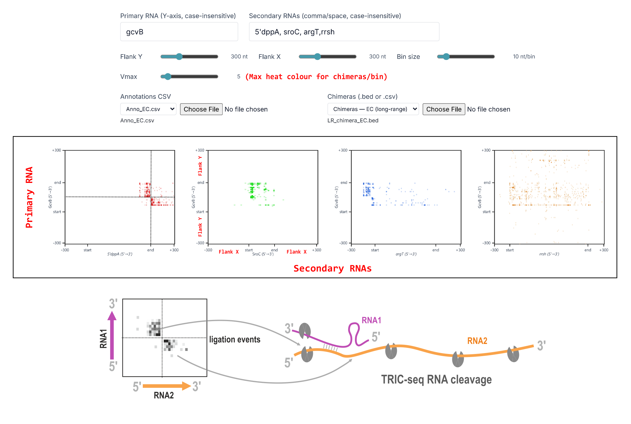
Pair lens ≈ pairMAP

What it shows: a high‑resolution base‑pairing contact map between the focal RNA (Y axis) and one chosen partner (X axis), both drawn 5′→3′. Choose the partner by double‑clicking it (in the Interactome or the partners list) or with the dropdown. Bright cells are nucleotide bins that ligated often — i.e. were in close contact.

Pair lens — base-pairing contact map between GcvB and the 5' UTR of oppA — Pair contact map for *GcvB* (Y) × the 5′UTR of *oppA* (X) — a textbook GcvB target. The contact hotspot pins the interface to GcvB's conserved R1 region; axis ticks mark −flank / start / end / +flank, colour = read depth, and the cross marks the predicted base‑pairing site.

Controls

Flank Y / Flank X — how much sequence (±nt) to show around each transcript (default ±300).
Bin — nucleotides per cell (default 10 nt). Large windows are auto‑coarsened to stay legible.
Vmax — the colour ceiling; auto by default, lower it to bring out faint signal.

Built‑in base‑pairing prediction

The Pair lens runs a lightweight, RNAduplex‑style predictor over ±30 nt of each feature and reports up to two candidate duplex sites: estimated ΔG, base‑pair count (including G·U), the nucleotide span in each RNA, and the alignment. Each site is drawn as a cross on the map (black = site 1, grey = site 2). When the cross lands on a TRIC‑seq hotspot, you have independent sequence support for that interface.

Read it as: a focused hotspot near the two interfaces → a base‑pairing interface (classic sRNA–5′UTR); a diffuse block across a CDS → co‑association/aggregation; a 5′UTR + 3′UTR signal can reflect tertiary folding bringing the ends together. Treat the predicted ΔG as an estimate (it approximates IntaRNA's seed but omits the accessibility term). Sequence prediction is available for the bundled species and the demo.

Structure lens ≈ foldMAP

What it shows: the focal RNA's intramolecular (self‑contact) map — an average picture of how the molecule folds back on itself in vivo — alongside a long‑range contact profile.

Structure lens for GcvB. Left: the symmetric self‑contact matrix (5′→3′ on both axes, gene body framed, flanks shaded). Right: the long‑range (> 5 kb) contact profile, with maxima marked.

Controls

Bin — nucleotides per cell (default 20 nt); smaller is sharper but sparser.
Flank — how much flanking sequence (±nt) to include (default 200).
raw / ICE — switch to ICE to balance per‑position coverage biases and bring out genuine architecture.
Vmax — colour ceiling (auto by default).

Read it as: blocks along the diagonal = local folded domains; gaps between blocks = insulated boundaries; off‑diagonal “corner” signal = long‑range contacts (e.g. 5′–3′ end pairing). The long‑range profile on the right counts contacts each position makes with loci > 5 kb away and flags the peaks — useful for spotting distal/trans engagement. This is a population average, so several conformations can overlay.

Compare lens ≈ csMAP

What it shows: the focal RNA's target spectrum placed side‑by‑side with any RNAs you've pinned. Pin partners with the pin icon in the partners list; the Compare tab badge tracks how many you've added.

Compare lens — target spectra of GcvB, 5'oppA, SroC and CsrB side by side — Compare lens: *GcvB* (focal) against its target *5′oppA*, its sponge *SroC*, and the unrelated sRNA *CsrB*. Each column's dots are that RNA's distal targets (y = odds ratio, area = reads, colour = target class); the lower panel shows total interactions per RNA (log scale) — GcvB's hub connectivity towers over the rest.

The scatter (top) lines up each RNA's enriched distal targets so you can compare partner classes and specificity at a glance.
The totals bars (bottom) compare overall connectivity — useful for separating promiscuous hubs from focused regulators.
The focal RNA is always the first, highlighted column.

Use it to contrast candidate hub sRNAs, or a regulator against a suspected sponge: similar target classes hint at shared logic; very different spectra argue for distinct roles.

Partners panel & export

The right‑hand panel is shared by every lens. At the top it summarises the focal RNA — feature type, coordinates, strand, total interactions and the number of partners passing your filters — with a link out to the relevant gene database (BioCyc, AureoWiki or SubtiWiki, by species).

Sort the partner list by Odds ratio, Reads, FDR, Distance or Position.
Click a row to refocus; double‑click (or the grid icon) to open its Pair map; the pin icon adds it to Compare; the ↗ icon opens it in a gene database.
Export CSV downloads the full partner table (partner, feature, coordinates, reads, odds ratio, FDR, distance).
AI hypothesis sends the high‑confidence partners (reads ≥ 5 and O^f ≥ 10) to a model that drafts a short, testable regulatory hypothesis — a starting point, not a conclusion.

Bring your own data

From the dataset menu, under Your data, upload an annotations CSV (gene_name, start, end, feature_type, strand, chromosome) and an interactions CSV (ref, target, counts, odds_ratio, fdr, totals, total_ref, ref_type, target_type). These power the Interactome, Compare and partners views immediately. The Pair and Structure contact maps rely on raw chimera files, which are bundled for the provided species and the demo.

Legacy standalone tools

The four original tools below are kept for reference and reproducibility. Everything they do is now available — and linked together — inside the Explorer, which is the recommended way to work. The mapping is: globalMAP → Interactome, pairMAP → Pair, foldMAP → Structure, csMAP → Compare.

globalMAP

What it shows: a genome‑aware, RNA‑centric map of all partners for a selected RNA. Points encode partner position, O^f, i_o, and feature type. The table includes quick links (↗) to external gene databases based on your selected annotation preset.

Select a dataset preset for your species.
Search for an RNA (e.g., sRNA RyhB or CDS uvrA).
Tune filters: min i_o, min O^f, and feature class.
Click a partner to recenter globalMAP on it.

csMAP

What it shows: collapsed (comparative) interaction profiles so you can place multiple RNAs side‑by‑side and compare partner spectra.

Select a species preset.
Add two or more RNAs to compare (e.g., hub sRNAs or candidate sponges).
Use differences in partner classes (5′UTR vs. CDS) to infer logic; copy candidate pairs to pairMAP for interface‑level inspection.

pairMAP

What it shows: a high‑resolution inter‑RNA heat map for a chosen pair (axes are nucleotide positions, binned).

Enter a Primary RNA and one or more Secondary RNAs.
Set Flank (±nt around each RNA) and Bin (nt/bin) for resolution.
Interpret:
- Focused hotspot near diagonal → base‑pairing interface (typical sRNA–5′UTR).
- Diffuse CDS‑wide signal → co‑association/aggregation (e.g., mRNA–mRNA).
- 5′UTR hotspot + 3′UTR signal can reflect tertiary folding bringing ends together (not necessarily a second binding site).

foldMAP

What it shows: an intramolecular (self‑contact) map capturing an RNA's average tertiary organization in vivo.

Select a species and an RNA.
Choose bin size to balance detail vs. sparsity.
Look for domains (blocks along the diagonal), insulated boundaries, and interaction islands/deserts.

Note: foldMAP summarizes a population‑average contact map; multiple conformations can overlay into the observed pattern. Use the export buttons to save the contact map and long‑range profile (SVG/CSV).